DeepMind’s AlphaTensor (blog, paper), introduced in October 2022, uses deep reinforcement learning to discover efficient algorithms for matrix multiplication. It has, perhaps understandably, not received the same level of attention as recent advances in generative AI. However, there are a few aspects of this work which make it a particularly interesting development in deep learning:

The complexity of the problem is rooted in its fundamental mathematical structure, not in extracting information from large empirical (i.e. social or physical) data sets such as text, image, or omics data.
The action space is much larger ($10^{10}\times$ larger!) than that of games like chess and Go, making it extremely challenging to search the game tree efficiently. The number of algorithms discovered demonstrates that this area is far richer than was previously understood.
AlphaTensor combines multiple state-of-the-art techniques to tackle the problem, including a transformer network to select actions from a high dimensional, discrete space and Monte Carlo tree search (MCTS) to solve the reinforcement learning problem.

In this post I break down the matrix multiplication problem and walk through my implementation of AlphaTensor. (Most figures below are from the AlphaTensor paper.)

Doing Arithmetic Efficiently

It may seem surprising that the standard way of doing matrix multiplication is not optimal, but this stems from two facts:

Multiplication is a more expensive operation than addition.
For large arithmetic calculations, there are many sequences of operations which produce the correct result.

To illustrate (1), try calculating each of the following in your head:

$$15047 + 30821$$ $$15047 \times 30821$$

It should be clear that multiplication is more work!

More precisely, consider two integers, each of $n$ digits (or bits). Using standard “pencil-and-paper” methods, the time complexity of adding them is $O(n)$ - we first add the digits in the ones place and carry, then those in the tens place, etc. The time complexity of multiplying them is $O(n^2)$ - we multiply the ones digit of the first number by every digit in the second number, then do the same for the tens digit, etc. Alternatively, if we denote the value of an integer as $N$ then addition is $O(log(N))$ and multiplication is $O(log^2(N))$. The key point is that the complexity of standard multiplication scales as the square of the complexity of addition. (However, faster multiplication algorithms exist which are $O(n \space log(n))$, still slower than addition.)

To illustrate (2), consider the example (courtesy of Assembly AI) of computing the difference of two squares, $a^2 - b^2$. Both of these algorithms produce the correct result:

$c_1 = a \cdot a$
$c_2 = b \cdot b$
return $c_1 - c_2$

$d_1 = a + b$
$d_2 = a - b$
return $d_1 \cdot d_2$

Though they each involve three operations, the latter only requires one multiplication and is faster. For matrix multiplication, there is a combinatorially large number of such “calculation paths” to consider.

Matrix Multiplication

Consider the matrix multiplication $C = AB$ where $A$ and $B$ are $2 \times 2$ matrices. (I’ll focus on this example, but the process is generalizable to any size matrices.)

\[\begin{pmatrix}c_1 & c_2\\\ c_3 & c_4\end{pmatrix} = \begin{pmatrix}a_1 & a_2\\\ a_3 & a_4\end{pmatrix} \cdot \begin{pmatrix}b_1 & b_2\\\ b_3 & b_4\end{pmatrix}\]

The standard way to compute this is:

\[c_1 = a_1b_1 + a_2b_3 \text{, etc.}\]

Each element of the product requires two multiplications, resulting in eight multiplications overall. In 1969, mathematician Volker Strassen showed that this can be computed using a method which requires only seven multiplications.

That’s a surprising result! But it probably also comes across as a clever one-off trick - it does not immediately suggest any structured approach to finding efficient algorithms for larger matrices. Can we do any better than blind trial-and-error or simple heuristics? We can! AlphaTensor is rooted in two observations which allow us to reframe this challenge as a problem of efficiently searching a game tree.

Matrix Multiplication can be Expressed as a Tensor

We can describe the multiplication $C=AB$ by a three-dimensional tensor $\mathcal{T}$ where the element $t_{ijk}$ denotes the contribution of $a_ib_j$ to $c_k$.

\[c_k = \sum_{i,j}{t_{ijk}a_ib_j}\]

The elements of $\mathcal{T}$ are all in $\{0, 1\}$ and we can visualize it by shading each of the non-zero elements:

Note that $c_1 = a_1b_1 + a_2b_3$ is denoted by:

$t_{111} = 1$
$t_{231} = 1$
$t_{ij1} = 0 \space \forall \space \text{other} \space (i, j)$
and similarly for $c_2$, $c_3$, and $c_4$.

Matrix Multiplication Algorithms are Tensor Decompositions

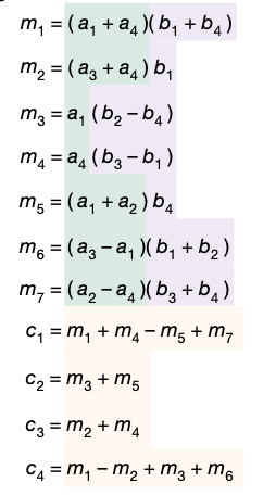
Strassen’s algorithm can be described as performing a sequence of actions, each of which has four parts:

Compute $u$, a linear combination of elements of $A$. (highlighted in green above)
Compute $v$, a linear combination of elements of $B$. (highlighted in purple above)
Compute the product $m=uv$.
Add $m$ (multiplied by a vector ${\bf w}$) to the elements of $C$. (highlighted in yellow above)

Each action involves one scalar multiplication and Strassen’s algorithm requires seven actions. It can be expressed more compactly by stacking these into three matrices $(U,V,W)$. Each column represents one action in an algorithm to compute $C$, defined by the column vectors $({\bf u}$, ${\bf v}$, ${\bf w})$.

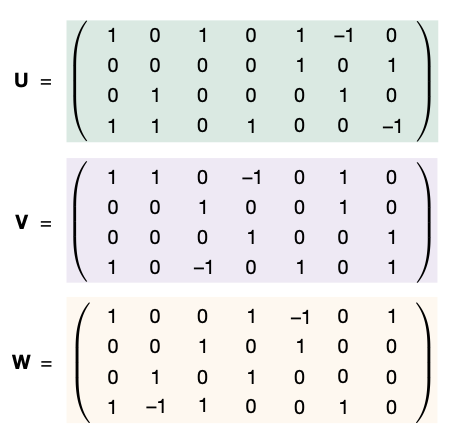
Now for the main trick - $(U,V,W)$ can equivalently be viewed as a tensor decomposition of $\mathcal{T}$. Here’s what this means: consider the zero tensor $\mathcal{S}=0$ of same dimensions as $\mathcal{T}$. For each set of factors $({\bf u}$, ${\bf v}$, ${\bf w})$, perform the following update to $\mathcal{S}$:

\[s_{ijk} \leftarrow s_{ijk} + u_iv_jw_k\]

After doing this for all seven columns we end up with $\mathcal{S}=\mathcal{T}$. Thus we can reframe the problem as a single player game whose goal is to find a sequence of actions which produces a low-rank decomposition of $\mathcal{T}$. (In practice, we set the initial state as $\mathcal{S}=\mathcal{T}$ and subtract $u_iv_jw_k$ at each step, so that the target state is always $\mathcal{S}=0$.) This is referred to as TensorGame and AlphaTensor is a method for learning to play this game.

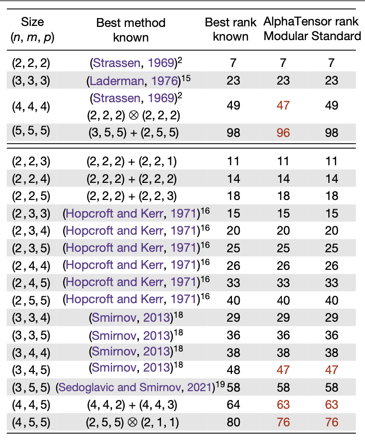
The table below shows the best results discovered by AlphaTensor for multiplication of various matrix sizes. Each row shows the number of actions (or rank) needed to multiply matrices of sizes $n \times m$ and $m \times p$. In each case, AlphaTensor was able to match or surpass the current best known algorithm - the paper even reports improvements up to size $(11, 12, 12)$. To be clear, the results themselves are not a groundbreaking improvement in computational efficiency. Rather, what is most impressive is that AlphaTensor demonstrates a promising method for searching extremely large combinatorial spaces which can be applied to many problems.

Implementing AlphaTensor

The approach of AlphaTensor is broadly as follows:

Build a model to choose an action $( {\bf u, v, w})$ and estimate a state-value $Q$, given a state $\mathcal{S}$.
Define a sufficiently dense reward function to provide feedback to the model.
Use a RL algorithm to explore the game tree for low-rank decompositions, guided by the model’s policy and value outputs.
Supplement the RL problem with a supervised learning problem on known decompositions.

In the rest of this post I’ll walk through the details of AlphaTensor. I’ll start with (2) and (4), as these are fairly straightforward. Next I’ll describe the model architecture for (1). Finally I’ll cover the Monte Carlo tree search algorithm used in (3) - this is not thoroughly described in the AlphaTensor paper and is fairly complex.

Reward function

Since the goal is to minimize the number of actions to reach a target state, AlphaTensor provides a reward of $-1$ for each action taken. Games are terminated when the target state is reached or after a finite number $(R_{limit})$ of steps. If $\mathcal{S}$ is still non-zero at this point, an additional reward of $-\gamma(\mathcal{S})$ is given, equal to “an upper bound on the rank of the terminal tensor” (code). In simpler terms, $\gamma(\mathcal{S})$ is roughly the number of non-zero entries remaining in $\mathcal{S}$ - we know that each of these could be eliminated by a single action. Note that this terminal reward plays an important role in creating a dense reward function. Without it, the agent would only receive useful feedback when it reaches the target state within $R_{limit}$ steps - which is effectively a sparse reward.

Supervised learning

While tensor decomposition is NP-hard, it is straightforward to do the inverse: to construct a tensor $\mathcal{D}$ from a given set of factors $\{({\bf u}^{(r)}, {\bf v}^{(r)}, {\bf w}^{(r)})\}^R_{r=1}$. This suggests a way to create synthetic demonstrations for supervised training - a set of factors is sampled from some distribution, and the resulting tensor $\mathcal{D}$ is given as an initial condition to the network, which is then trained to output the correct factors (code). AlphaTensor generates a large dataset of such demonstrations and uses a mixed training strategy, alternating between training on supervised loss on the demonstrations and reinforcement learning loss (learning to decompose $\mathcal{T}$). This was found to substantially outperform either strategy separately.

Network Architecture and Training

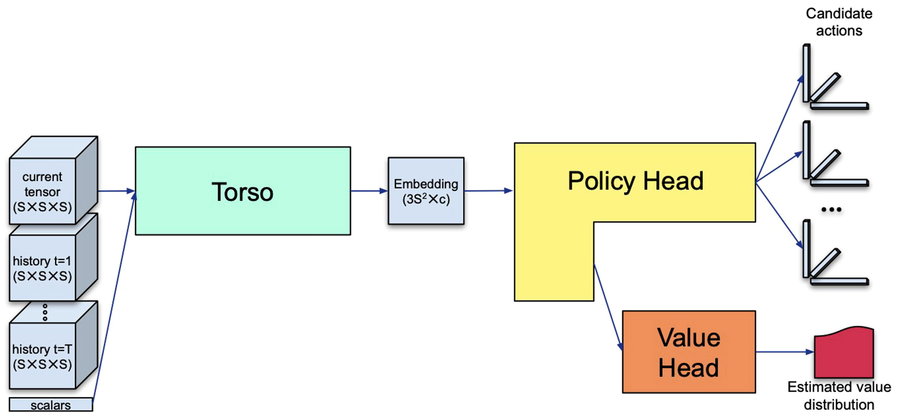
The AlphaTensor network consists of three components:

A torso (code), which takes information about the current state $\mathcal{S}$ and produces an embedding.
A policy head (code), which takes the embedding produced by the torso and generates a distribution over candidate actions.
A value head (code), which takes the embedding produced by the torso and generates a distribution of expected returns.

In the rest of this section I’ll give a brief overview of the architecture with links to my implementation. The network is quite complex (particularly the torso) and I won’t attempt to cover all the details - to fully understand it I recommend both the paper and the pseudocode provided in the Supplementary Information.

Training Process

The network is trained on a dataset which initially consists of synthetic demonstrations. Training is done by teacher-forcing - loss is computed for each action in the ground-truth training sequence given the previous ground-truth actions. Note that loss is computed both for the policy head (based on the probability assigned to the next ground-truth action) and for the value head (comparing the output value distribution to the ground-truth rank of the current tensor state).

Periodically (after a given number of epochs), MCTS is performed, starting from $\mathcal{T}$. This is the step in which we actually use the model to explore and look for a solution to the problem we are interested in. Note that MCTS uses both the policy and value heads in deciding which directions to explore. All of the played games are added to a buffer, while the game with the best reward is added to a separate buffer. Both of these buffers are merged with the training dataset and eventually training is performed on fixed proportions of synthetic demonstrations, played games, and “best” played games.

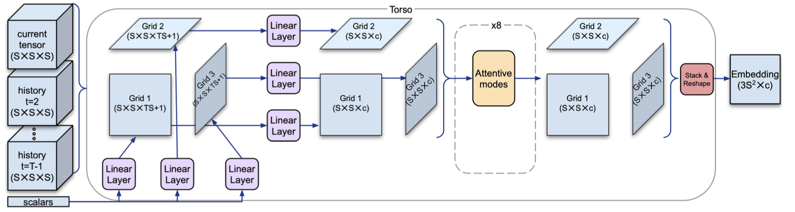
Torso

The torso converts the current state $\mathcal{S}$ (to be more precise, the past $n$ states in the game), as well as any scalar inputs (such as the time index of the current action), to an embedding that feeds into the policy and value heads. It projects the $4 \times 4 \times 4$ tensor onto three $4 \times 4$ grids, one along each of its three directions. Following this, attention-based blocks (code) are used to propagate information between the three grids. A block has three stages - in each stage one of the three pairs of grids is concatenated and axial attention is applied. The output of the final block is flattened to an embedding vector which is the output of the torso.

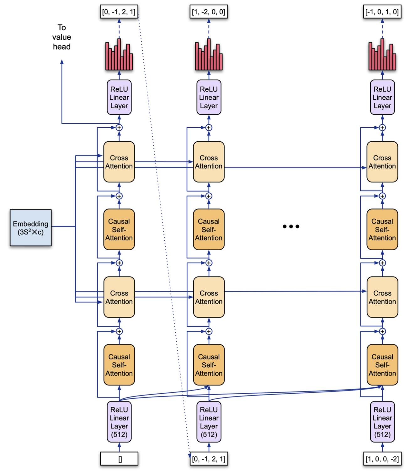
Policy Head

The policy head is responsible for converting the torso’s output into a distribution over the action space of the factors $( {\bf u, v, w})$ which we can run backpropagation on (during the training step) and sample from (during the action step used in MCTS). However, this action space can be too large for us to represent the distribution explicitly. Consider multiplication of $5 \times 5$ matrices. In this case each factor is of length $25$. In the AlphaTensor paper, entries in the factors are restricted to the five values $(-2, -1, 0, 1, 2)$ and the cardinality of the action space is $5^{3 \cdot 25} \approx 10^{52}$.

The solution is to use a transformer architecture to represent an autoregressive policy (code). In other words, an action is produced sequentially, with each token in the factors drawn from a distribution that is conditioned on the previous tokens (via self-attention), as well as on the embedding produced by the torso (via cross-attention). Naively, we might treat each of the $75$ entries in the three factors as a token. However, now we have moved from an enormous action space to the opposite extreme, a transformer with a vocabulary size of only $5$. Recall that transformers learn embeddings for each “word” in the vocabulary- the benefit of this is most apparent for large vocabularies. Note that we can represent sequential data using different n-gram representations which trade off between vocabulary size and sequence length. In this example, we can split the factors into chunks of 5 entries (5-grams) and represent each chunk as a token. With this approach, the vocabulary size (i.e. the number of distinct values a chunk can take on) increases to $5^5 = 3125$ and the sequence length decreases from $75$ to $15$. This vocabulary size is still small enough to learn embeddings over, but we have also reduced the context length that the transformer must learn to attend to.

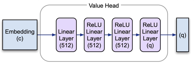
Value Head

The value head is a multilayer perceptron whose output is an estimate of the distribution of returns from the current state. This is expressed as a series of evenly spaced quantile values. The value head is trained against ground truth values using quantile regression (code, reference).

Monte Carlo Tree Search

So far we’ve described our network architecture and a method of training it on synthetic demonstrations. But how do we actually play TensorGame and search for low-rank decompositions? AlphaTensor uses MCTS, as described in the AlphaZero and Sampled MuZero papers. MCTS uses the output of the network’s policy and value heads, along with an upper-confidence bound decision rule to explore the game tree. The implementation of MCTS (code) involves a fairly deep call stack, with several nested loops and can be difficult to grasp from reading the code directly. We’ll build some intuition by illustrating this graphically.

To start - the purpose of the MCTS step is to generate a set of games (or trajectories) which will be added to the training dataset (as mentioned above). Also, of course, this is the step in which we are hoping to discover a low-rank decomposition! Naively, we might consider producing a trajectory by sequentially sampling actions from the policy head and updating $\mathcal{S}$. Perhaps we could generate several trajectories and add the best ones to the training buffer? Unsurprisingly, this simple approach is inefficient and MCTS offers a way to do better. It works by building a search tree (in which the nodes are states and the edges are actions) and using a decision rule to decide which branches to explore further, before finally choosing which action to take from the root state. Let’s break it down:

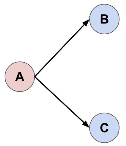
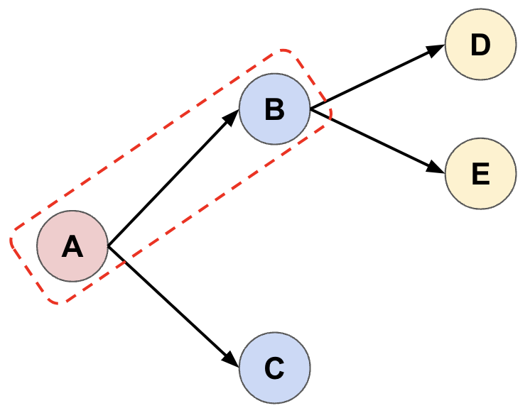
Initialize a tree with our initial state $A$ as the root. We next wish to extend the tree which we do by sampling $n_{samples} = 2$ actions from our network (code), given input state $A$. These actions produce the child states $B$ and $C$.
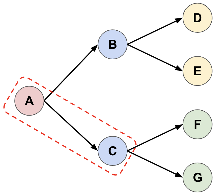
To continue extending the tree we must choose which leaf node ($B$ or $C$) to extend. We do this by starting at $A$ and using a decision rule (which I explain below) to traverse the tree. In this example, the rule selects the branch $A \rightarrow B$ (code). As above, we sample $n_{samples}$ actions at state $B$, extending the tree to $D$ and $E$.
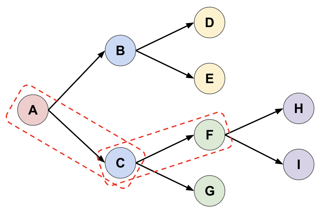
We repeat the process in (2), and this time our decision rule selects $A \rightarrow C$ instead (we’ll see why below) and we now extend the tree from $C$.
In the next iteration, we must apply the decision rule twice to reach a leaf node, selecting $A \rightarrow C$ followed by $C \rightarrow F$, before extending the tree from $F$.
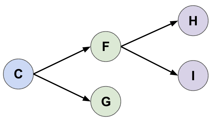
Continue until we have extended the tree $n_{sim}=4$ times. At this point, we are done exploration and will choose which action to take from $A$. We do this using the decision rule again. In this illustration we select $A \rightarrow C$ as the first action in our trajectory.
We now repeat the same process, starting from $C$ to choose the next action in our trajectory. Rather than build a new tree from scratch, we start with the subtree below $C$ and extend it until it has $n_{sim}$ branch nodes.

The decision rule used above (code) selects the action $a$ which maximizes the following quantity:

\[Q(s,a) + c(s) \cdot \hat{\pi}(s,a) \frac{ \sqrt{\sum_b{N(s,b)}}}{1 + N(s,a)}\]

where

$Q(s,a)$ - an action value, based on the upper quantiles of the value head output.
$N(s,a)$ - the number of MC visits to the state-action pair $(s,a)$
$\hat{\pi}(s,a)$ - empirical policy, the fraction of sampled actions from $s$ that were equal to $a$.
$c(s)$ an exploration factor to balance the two terms (essentially a hyperparameter)

This is an upper-confidence tree bound - it favors actions which have a high value but have not been explored frequently and have a high empirical policy probability.

Each time the tree is extended we do a backward pass (code) in which $N(s,a)$ and $Q(s,a)$ are updated for all nodes along the simulated trajectory.

DeepMind’s MCTS procedure uses $n_{samples}=32$ and $n_{sim}=800$, producing trees with up to 25,600 nodes. Given the enormous action space (up to $10^{12}$ actions), this is a very small subset of the full game tree!

Policy Improvement

Using the above steps, we can generate a MCTS trajectory. We can represent this trajectory as a sequence of actions, as well as the policy probability and value of each action: $\{(a_i, \hat{\pi}(a_i), Q(a_i)\}$

We use $\hat{\pi}(a_i)$ and $Q(a_i)$ as target values to train the policy and value heads respectively. In other words, the network is trained to select action $a_i$ not with probability 1, but with probability $\hat{\pi}(a_i)$.

A simple approach is to use $\hat{\pi}(a) = N(s,a)/N(s)$ as the policy, in other words the fraction of simulations from state $s$ which visit action $a$. Instead, AlphaTensor uses a temperature smoothing scheme to compute an improved policy (code):

\[\mathcal{I}\hat{\pi}(s,a) = \dfrac{[N(s,a)]^{1/\tau(s)}}{\sum_b{[N(s,b)]^{1/\tau(s)}}}\]

where $\tau(s)=\text{log }N(s)/\text{log }\bar{N}$ if $N(s)>\bar{N}$, else $1$.

Additional Details

The AlphaTensor paper includes some additional details which I did not implement. For completeness I mention them here:

Change of basis: $\mathcal{T}$ is expressed in a large number of randomly generated bases and AlphaTensor plays games in all bases in parallel.
Modular arithmetic: Agents are trained using either standard arithmetic or modular arithmetic.
Multiple target tensors: A single agent is trained to decompose tensors of different sizes. Since the network takes fixed-size inputs, smaller tensors are padded with zeros.