Summary

\(pass@k\) is widely used for open-ended, verifiable benchmarks (e.g. code, formal proofs), but its nonlinear dependence on both \(k\) and temperature \(T\) makes it difficult to reason about. I use a toy model to study this dependence and find:

The optimal temperature \(T^*\) (that which maximizes \(\mathbb{E}[\text{pass@k}]\)) depends on \(k\). \(T^*(k)\) follows a power law over several decades of \(k\).
- This behavior arises because eval sets contain tasks of varying difficulties (a “difficult task” being one with a low \(pass@1\)). For a single task, \(T^*\) is independent of \(k\).
- As \(k \rightarrow \infty\), \(T^*\) has an asymptotic upper bound that depends only on the single most difficult task in the eval set. For an infinite eval set (in other words, a task generating distribution) with no upper bound on task difficulty, the power law scaling would continue indefinitely.
The scaling exponent of \(T^*(k)\) is governed by the tail of the task difficulty distribution - not its mean or variance. Gaussian, exponential, and power-law difficulty distributions yield qualitatively different \(T^*(k)\) behavior, even when matched on the first two moments. Concretely, the \(k\)-exponent increases from 0.73 (Gaussian) to 1.05 (exponential), meaning temperature should scale roughly linearly with \(k\) for exponential difficulty distributions but sub-linearly for Gaussian ones. The plots below show \(T^*(k)\) curves for increasingly fat-tailed eval distributions (Gaussian < exponential < power law).

Motivation

Unlike greedy accuracy (binary per task, insensitive at low solve rates) or perplexity (dependent on a specific reference solution), \(pass@k\) is continuous-valued, increases with \(k\), and can be estimated to arbitrary precision.

However, \(pass@k\) introduces challenges that simpler metrics avoid:

Sensitivity to temperature: using \(T=0\) for \(k>1\) is suboptimal since all generations will be identical. It is not clear which \(T\) optimizes \(pass@k\), or whether comparing two models at the same \(T\) is apples-to-apples. (Model A may beat model B at \(T=0.5\) while model B wins at \(T=1\).)
Sensitivity to k: \(pass@k\) is a curve over \(1 \leq k < \infty\). It is not obvious whether a particular set of \(k\) values provides the full picture when comparing two models.
Nonlinear interaction: \(pass@k\) has a nonlinear dependence on \(k\) and \(T\) that cannot easily be factored into independent effects, making it difficult to reason about analytically.

I developed a toy model to isolate how \(pass@k\) depends on \(k\), \(T\), and the distribution of task difficulties across an eval set. The key questions:

For a single task, \(pass@k = 1 - (1-pass@1)^k\). But we report the average over a benchmark - how does the \(pass@k\) curve behave for a set of tasks with varying difficulty?
For a given \(k\), there is an optimal \(T\) that maximizes \(pass@k\) (an exploration vs. exploitation trade-off). How does \(T^*(k)\) scale?
Does the shape of the task difficulty distribution matter, beyond its mean and variance?

Toy Model

For any task prompt, assume there is some non-zero probability (at \(T>0\)) that a given LLM will generate a correct solution. The probability of generating a specific token \(x_i\) scales with \(T\) as:

\[p(x_i) \sim \exp(z_i / T)\]

(where \(T\) also influences the normalization constant). Note the similarity to a zero-mean normal distribution:

\[p(x) \sim \exp(-x^2 / 2 \sigma^2)\]

Consider a discrete normal distribution (i.e. defined only on the integers \(\mathbb{Z}\)). This is equivalent to a softmax function over \(\mathbb{Z}\) where \(z_i = -x_i^2 / 2\) and \(T = \sigma^2\).

Since the possible generations of an LLM form a countable set, we can view this distribution as a simplified representation of an LLM (where each integer represents one generation). A task is represented by an integer \(c\): we sample a random integer \(g\) from the model distribution and say it passes if \(g=c\). Tasks with large \(\lvert c \rvert\) are “difficult” (low probability under the model) and tasks with small \(\lvert c \rvert\) are “easy.”

The model intentionally strips away semantic content to isolate the dependence of \(pass@k\) on temperature, sample count, and the distribution of task difficulties. The absence of task-specific prompts (i.e. we always generate from the same distribution) is not a limitation - what matters is that each task has a \(pass@1\) rate of \(p_{gen}(c \mid T)\) that depends on its difficulty \(\lvert c \rvert\) and the temperature \(T\).

The final element is the evaluation set \(\{c_i\}\). The task difficulties are sampled from a distribution \(p_{task}(c)\) (not to be confused with the generation distribution \(p_{gen}\)). I consider three families:

Task distribution	Form	Key parameter
Gaussian	\(p_{task}(c=j) \sim \exp(-j^2 / 2\sigma_{task}^2)\)	\(\sigma_{task}\) (task_spread)
Exponential	\(p_{task}(c=j) \sim \exp(-\lvert j \rvert / \sqrt{T_{task}})\)	\(T_{task}\)
Power law	\(p_{task}(c=j) \sim \lvert j \rvert^{-\gamma}\)	\(\gamma\)

These families have increasingly fat tails, allowing us to test whether the tail shape - independent of the first two moments - affects the scaling of \(T^*(k)\).

Results

Temperature dependence for a single task

Before examining eval sets, it is useful to understand how \(pass@1\) depends on \(T\) for a single task. For \(p_{gen}(c \mid T)\):

At \(T=0\), \(p_{gen}(c)=0\) unless \(c\) is the maximum-likelihood generation.
As \(T\) increases, probability mass initially spreads from the mode toward \(c\), increasing \(p_{gen}(c \mid T)\).
Increasing beyond some optimal \(T\), more mass flows away from \(c\) toward the tails than flows to \(c\) from the mode, and \(p_{gen}(c \mid T)\) decreases.
Concretely, for a zero-mean normal distribution, \(p(x)\) is maximized when \(\sigma = \lvert x \rvert\). The plot below illustrates this - compare the values of each curve at \(x=1\):

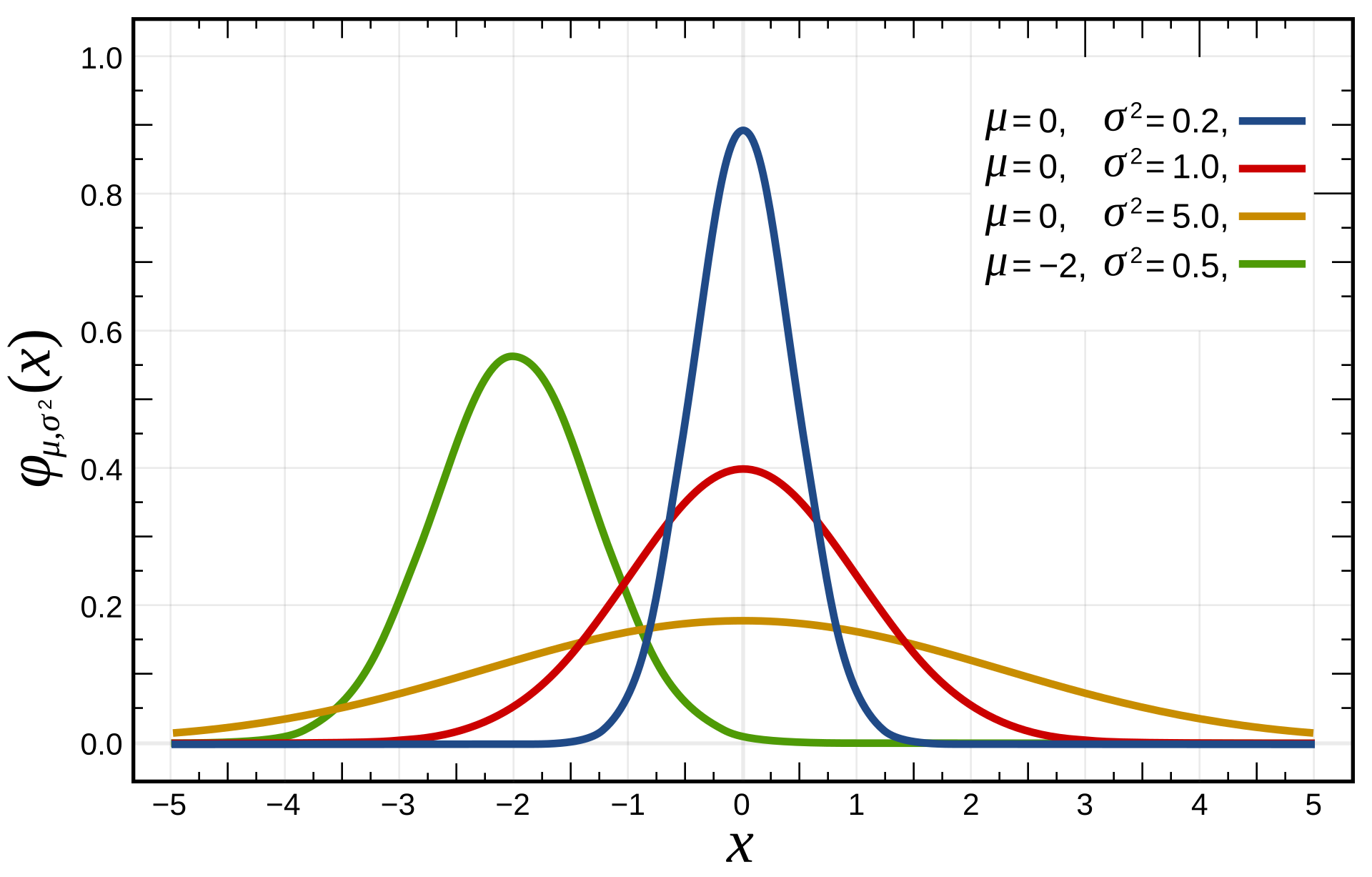
For a single task, this optimal \(T\) is independent of \(k\) (since \(pass@k = 1-(1-pass@1)^k\) is monotonically increasing in \(pass@1\)).

How does \(T^*\) scale with \(k\) for an eval set?

For a set of tasks the answer is different. I created eval sets by sampling tasks from each distribution family and calculated \(T^*(k)\) - the temperature maximizing \(pass@k\) for each \(k\) - using Brent’s method.

Key observations:

As \(k \rightarrow \infty\), \(pass@k\) is dominated by the most difficult task (the largest \(\lvert c \rvert\)). Asymptotically, \(T^*\) converges to the value that maximizes \(pass@1\) for that task. This asymptotic value is noisy since it depends on a single extreme task.
For intermediate values of \(k\), \(T^*\) follows a smooth power law over several decades - this is the scaling regime I focus on.

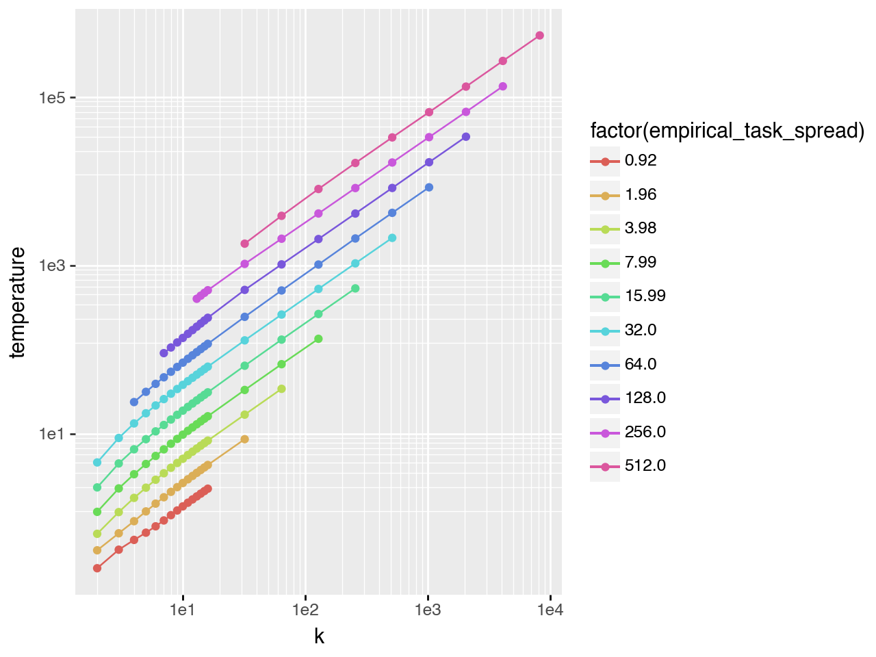
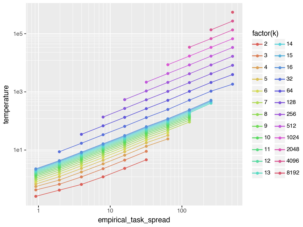
Gaussian task difficulty

The left plot shows the full \(T^*\) vs \(k\) curve (\(task\_spread\) is the standard deviation of the task distribution). The right plot shows only points with \(0.03 < pass@k < 0.98\), isolating the scaling regime. The bottom plot shows that \(T^*\) also follows a scaling law with respect to \(task\_spread\).

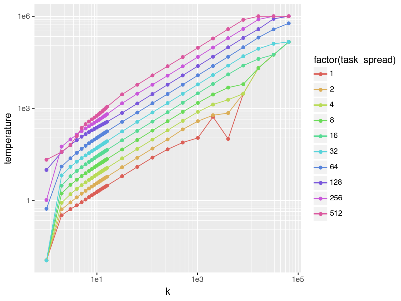
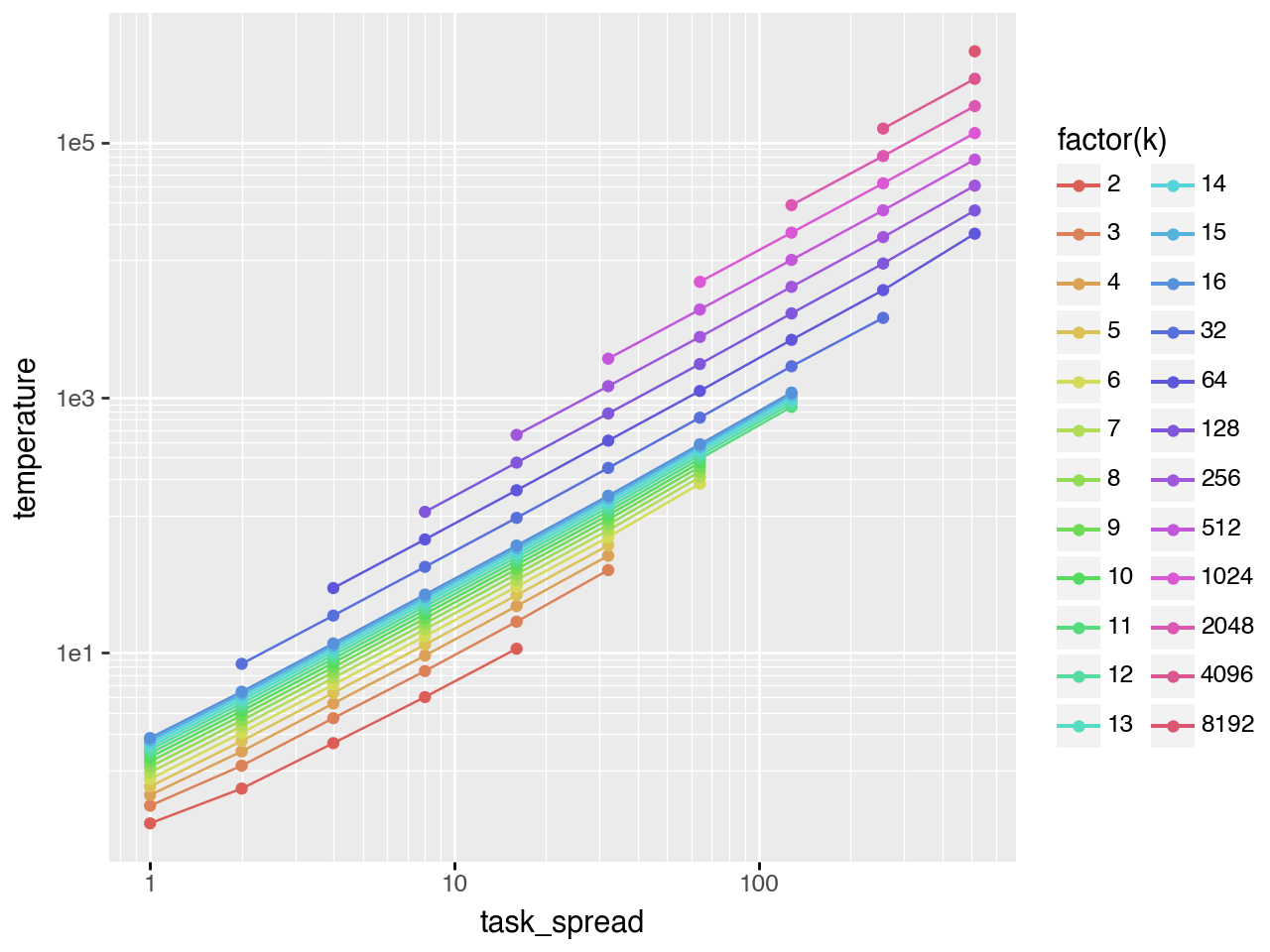
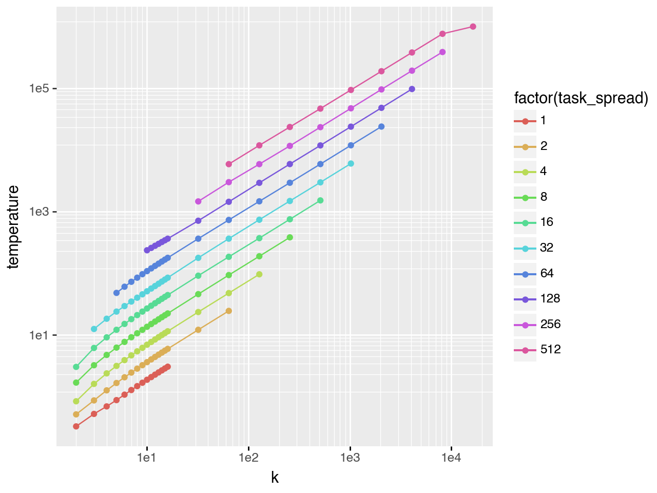
Fitting a regression in this scaling regime (s = task_spread):

\[T^* \approx 0.264 \cdot k^{0.728} \cdot s^{1.283} \text{ ; } R^2=0.9996\]

Exponential task difficulty

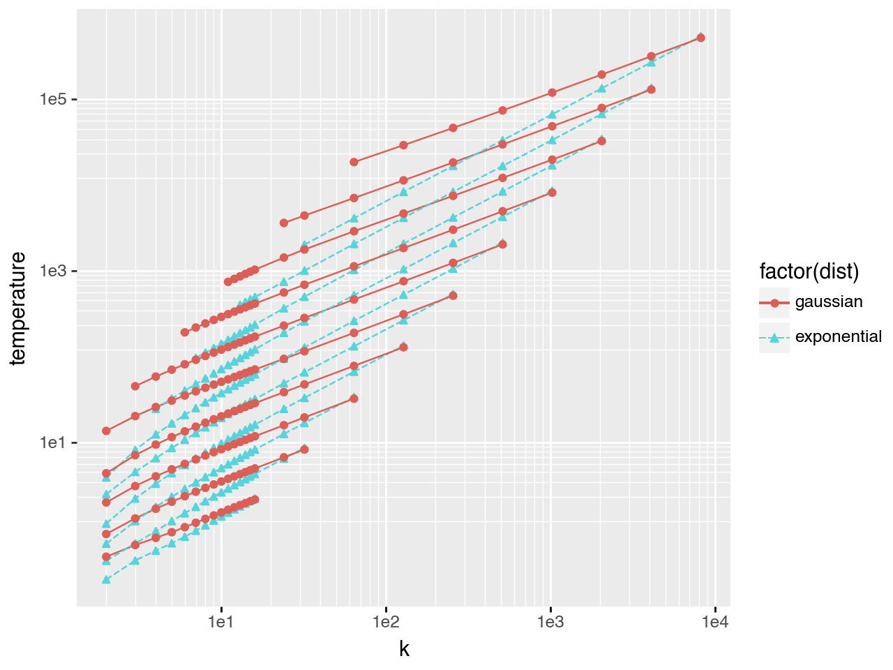
The same analysis with tasks drawn from an exponential distribution yields different scaling exponents:

\[T^* \approx 0.117 \cdot k^{1.054} \cdot s^{0.957} \text{ ; } R^2= 0.9989\]

The \(k\)-exponent increases from 0.73 to 1.05 - temperature must scale approximately linearly with \(k\) for exponentially-distributed task difficulties, compared to sub-linearly for Gaussian. This points to the central finding: the optimal temperature for a given eval set does not only depend on the mean and variance of the task difficulty distribution - it depends on the form of the tail. Two eval sets with identical first and second moments but different tail shapes will require qualitatively different temperature-scaling strategies as \(k\) grows.

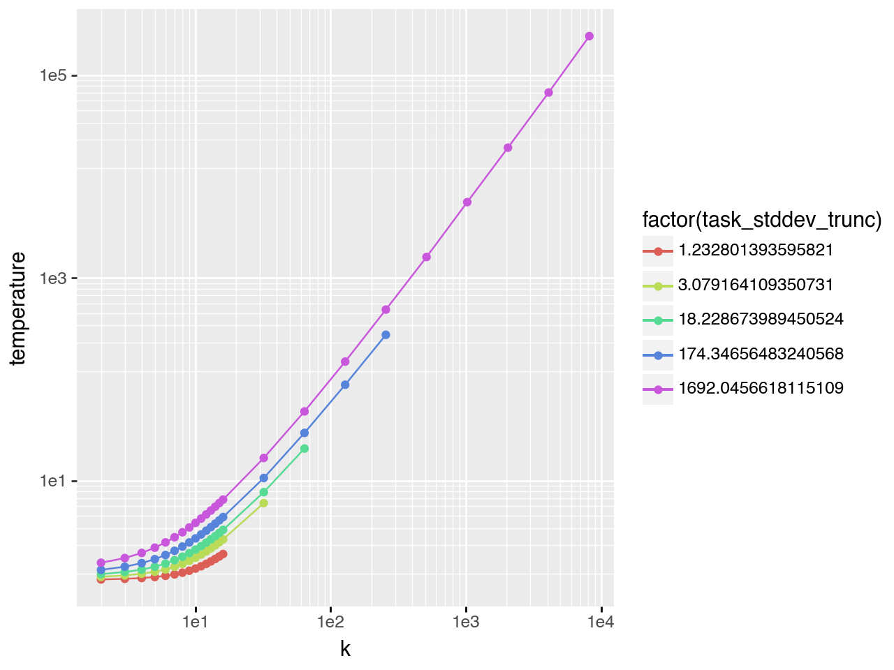
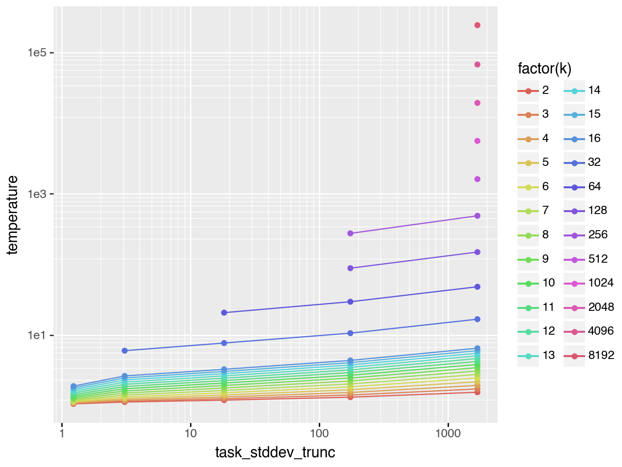
Power-law task difficulty

Power-law distributions have even fatter tails, providing a further test of this finding. Here the scaling behavior with respect to \(k\) does not appear at low \(k\) and low \(pass@k\) rates - it only emerges at \(k \approx 20\). (Note: task_stddev_trunc is the equivalent of task_spread here, calculated from the actual truncated distribution since truncation has a much stronger effect on power-law than on Gaussian/exponential distributions.)

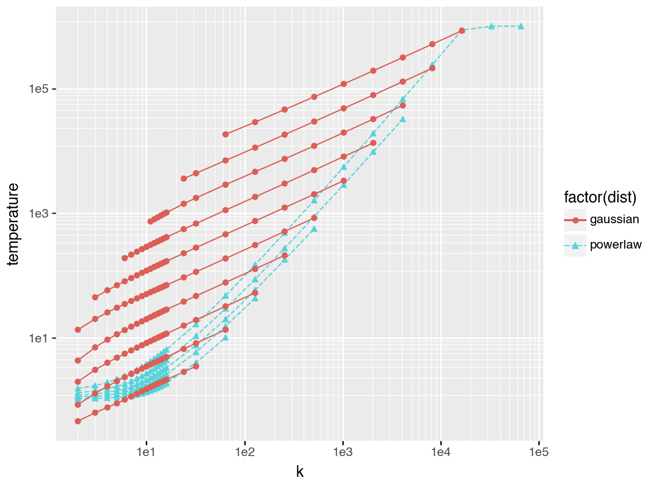
Comparing all three task distributions

The plots below overlay \(T^*(k)\) for all three distribution families. Gaussian and power-law task sets can have similar \(pass@k\) for \(k<10\), but diverge sharply at larger \(k\). Performance on the Gaussian set saturates by \(k \sim O(100)\), requiring only a modest increase in \(T\) to pass the hardest tasks. For the power-law set, \(T\) must increase by several orders of magnitude to reach the hardest tasks, and even then \(pass@k\) rises slowly with \(k\).

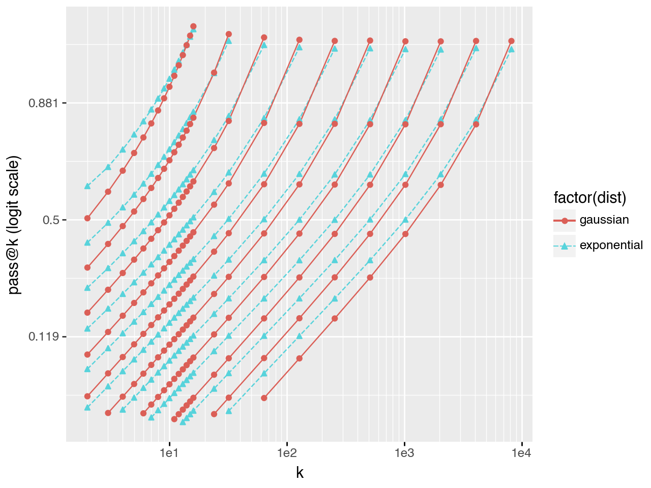
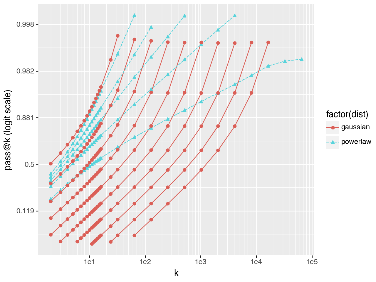
Deciding how large to make k

When planning experiments it is useful to estimate the minimum \(k\) necessary to reach a desired \(pass@k\) score. Comparisons between models are most informative when \(pass@k\) values are near 0.5 rather than clustered near 0 or 1. The plots below show that in many cases there is a linear relationship \(\log(k) \sim \text{logit}(pass@k)\). This suggests that \(pass@k\) for large \(k\) can be extrapolated from a small number of samples, substantially reducing compute requirements.

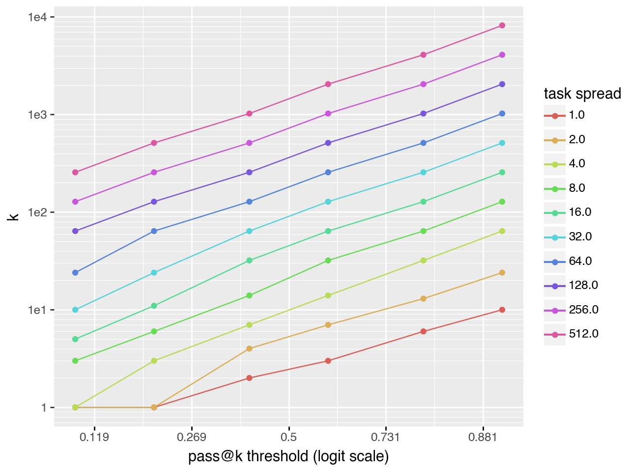
Gaussian task distribution

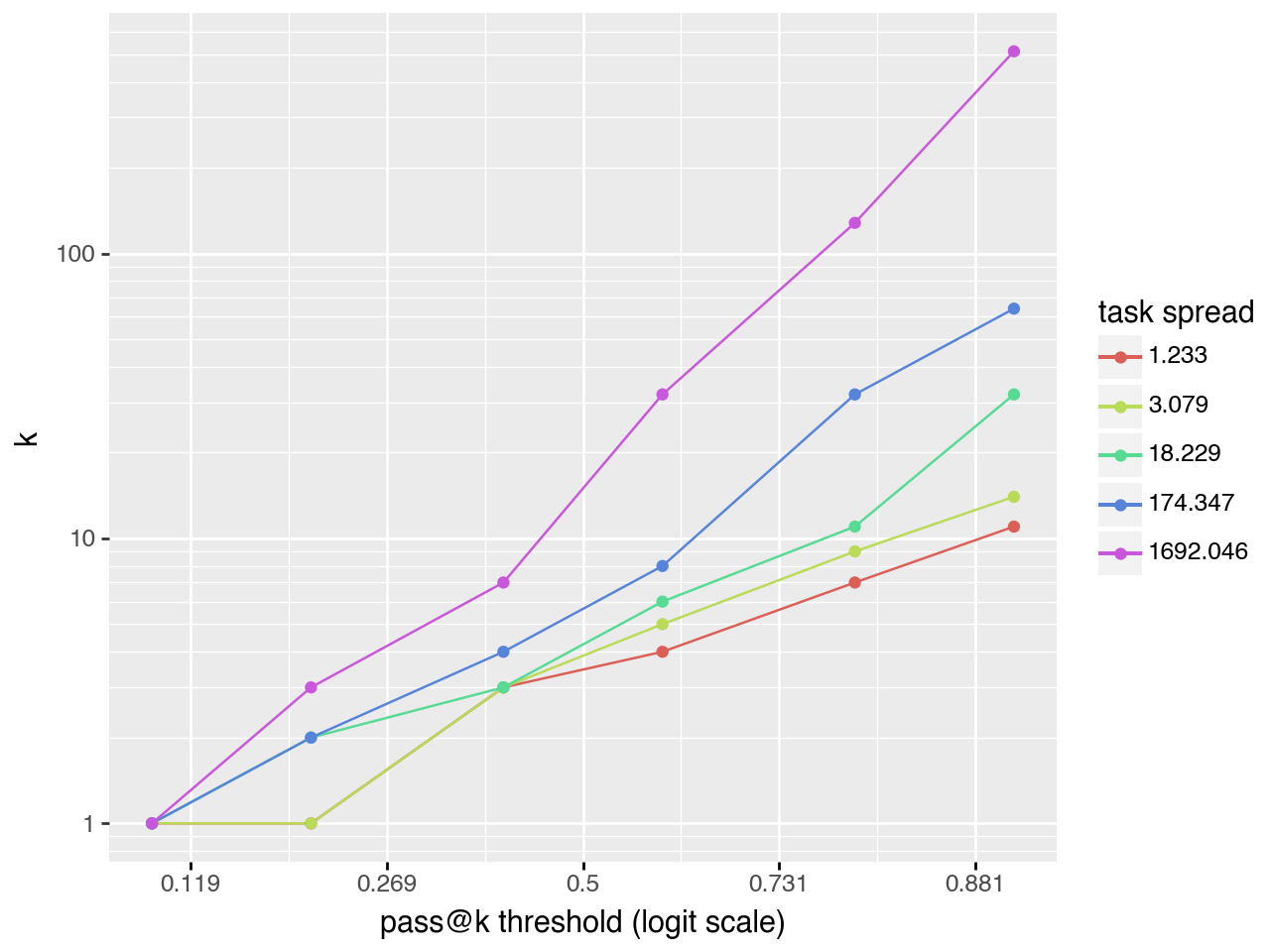
Exponential task distribution

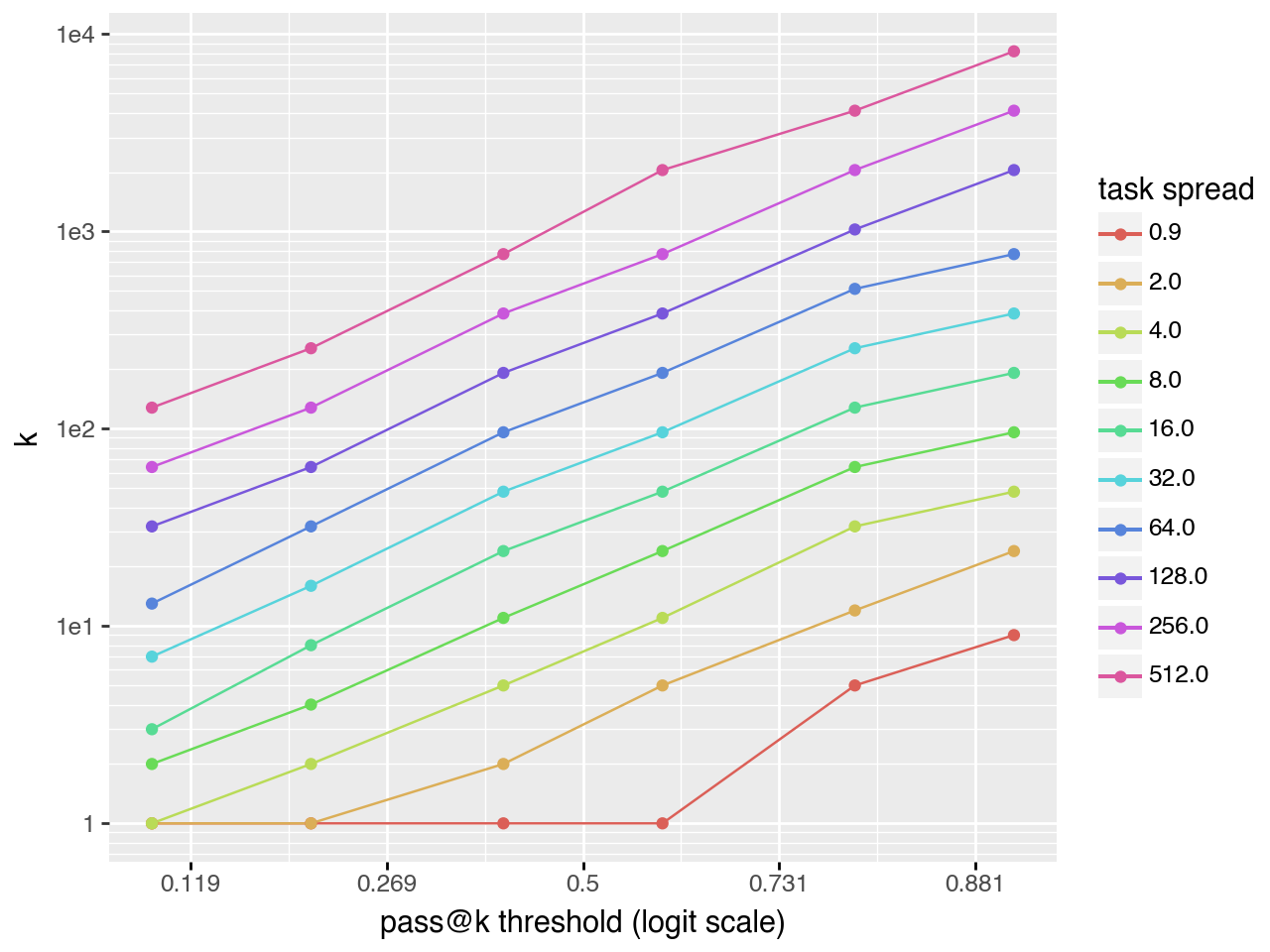
Power law task distribution

Implications

The main practical takeaways from this analysis:

Temperature tuning for pass@k should account for the difficulty distribution of the eval set. Using a fixed temperature across benchmarks with different tail characteristics will be systematically suboptimal. Fat-tailed benchmarks (where a few tasks are much harder than the rest) require substantially higher temperatures at large \(k\).
The \(k\)-exponent of \(T^*(k)\) serves as a fingerprint of the eval set’s difficulty distribution. Measuring this exponent on a real benchmark could reveal whether its difficulty distribution is closer to Gaussian, exponential, or power-law - information that is otherwise hard to extract.
Extrapolating pass@k via the log-logit relationship could reduce the number of generations needed to estimate performance at large \(k\), making high-\(k\) evaluation more practical.
When comparing models on pass@k, the choice of \(k\) and \(T\) is not neutral. Two models may rank differently depending on these choices, and the degree to which rankings are sensitive to \((k, T)\) depends on the tail of the benchmark’s difficulty distribution.